Spatial mapping to tranfer cell type labels and expression values

In this tutorial, we will demonstrate how CellMapper can be used to transfer labels and expression values from a dissociated reference to a spatial query dataset.

Along the way, we’ll use squidpy [PSK+22] for plotting and Harmony [KMF+19] to compute a joint latent representation between spatial and dissociated data.

Preliminaries

Import packages & data

%load_ext autoreload
%autoreload 2

import matplotlib.pyplot as plt
import warnings
import scanpy as sc
import squidpy as sq
import anndata as ad
from harmony import harmonize
import cellmapper
import seaborn as sns
import numpy as np

sc.set_figure_params(scanpy=True, frameon=False, fontsize=14)

Load the seqFISH data of [LGM+22] as a spatial query dataset and the scRNA-seq data of [PSGG+19] as a dissociated reference dataset. Both profile mouse embryogenesis at approximately embryonic day (E) 8.5.

ad_sp = sc.read("data/spatial_data.h5ad", backup_url="https://figshare.com/ndownloader/files/54145250")
ad_sp

AnnData object with n_obs × n_vars = 51787 × 351
    obs: 'embryo', 'pos', 'z', 'embryo_pos', 'embryo_pos_z', 'Area', 'celltype_seqfish', 'sample_seqfish', 'umap_density_sample', 'modality', 'total_counts', 'n_counts', 'celltype_harmonized'
    uns: 'celltype_harmonized_colors', 'celltype_seqfish_colors', 'embryo_colors', 'pca', 'umap'
    obsm: 'X_pca', 'X_umap', 'X_umap_orig', 'spatial'
    varm: 'PCs'

ad_diss = sc.read("data/dissociated_data.h5ad", backup_url="https://figshare.com/ndownloader/files/54145217")
ad_diss

AnnData object with n_obs × n_vars = 16496 × 18499
    obs: 'barcode', 'sample_rna', 'stage', 'sequencing.batch', 'theiler', 'doub.density', 'doublet', 'cluster', 'cluster.sub', 'cluster.stage', 'cluster.theiler', 'stripped', 'celltype_rna', 'haem_subclust', 'endo_trajectoryName', 'endo_trajectoryDPT', 'endo_gutDPT', 'endo_gutCluster', 'sizefactor', 'modality', 'total_counts', 'n_counts', 'celltype_harmonized'
    var: 'gene_ids', 'n_cells', 'highly_variable', 'means', 'dispersions', 'dispersions_norm'
    uns: 'celltype_harmonized_colors', 'celltype_rna_colors', 'cluster_colors', 'hvg', 'pca', 'sample_colors', 'sequencing.batch_colors', 'stage_colors', 'theiler_colors', 'umap'
    obsm: 'X_endo_gephi', 'X_endo_gut', 'X_haem_gephi', 'X_pca', 'X_umap', 'X_umap_orig'
    varm: 'PCs'

The spatial data contains all genes measured with seqFISH, the dissociated data contains all genes that passed basic filtering criteria. In both objects, .X corresponds raw counts. We manually harmonized cell type annotations (stored in .obs["celltype_harmonized"] in either object), following ENVI [HRemvsikG+25].

Basic preprocessing

Later on, we will want to evaluate the sucess of expression imputation. For that, let’s annotate genes as either test or train.

n_test_genes = 50
rng = np.random.default_rng(seed=0)

# annotate test genes
shared_genes = set(ad_diss.var_names).intersection(set(ad_sp.var_names))
test_genes = rng.choice(list(shared_genes), replace=False, size=n_test_genes)
train_genes = list(shared_genes - set(test_genes))

# format as .var columns
for adata in [ad_sp, ad_diss]:
    for key, genes in zip(["is_train", "is_test"], [train_genes, test_genes], strict=False):
        adata.var[key] = False
        adata.var.loc[genes, key] = True

print(f"Using {len(test_genes)} genes for testing and {len(shared_genes) - len(test_genes)} for training.")

Using 50 genes for testing and 300 for training.

Let’s also do basic normalization of both objects

ad_sp.layers["counts"] = ad_sp.X.copy()
sc.pp.normalize_total(ad_sp, target_sum=1e4)
sc.pp.log1p(ad_sp)

ad_diss.layers["counts"] = ad_diss.X.copy()
sc.pp.normalize_total(ad_diss, target_sum=1e4)
sc.pp.log1p(ad_diss)

Basic visualization

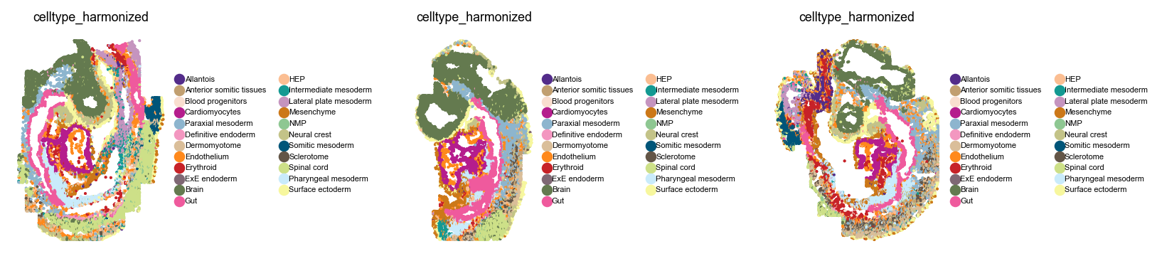
Let’s take a closer look at these two datasets before we get started. For the seqFISH data, we can visualize harmonized cell type labels in space.

with warnings.catch_warnings():
    warnings.simplefilter("ignore")

    with plt.rc_context({"figure.figsize": (2, 2.5), "legend.fontsize": 5, "axes.titlesize": 8}):
        sq.pl.spatial_scatter(
            ad_sp,
            library_key="embryo",
            color="celltype_harmonized",
            shape=None,
            wspace=0.8,
        )

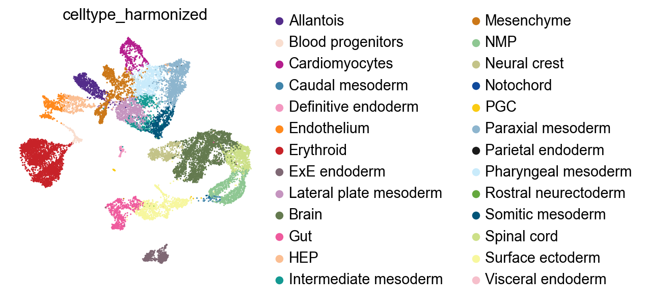
For the dissociated data, we can show a simple UMAP.

sc.pl.embedding(ad_diss, basis="X_umap", color="celltype_harmonized")

Compute a joint embedding

Everything we do in CellMapper is based on a joint embedding between query (spatial) and reference (dissociated) data. For simplicity, we will compute such a joint embedding here with Harmony [KMF+19].

Note that we’re using mask_var="is_train" to compute the PCA, which holds out test genes for the PCA, and for Harmony, which is based on the PCA. Thus, test genes will be masked for all downstream computations, because they all depend on the joint latent space.

# let's define batch labels in both objects
ad_sp.obs["batch"] = ad_sp.obs["embryo"].copy()
ad_diss.obs["batch"] = ad_diss.obs["sample_rna"].copy()

# Harmony expects a combined AnnData object and a joint PCA
ad_combined = ad.concat(
    [ad_sp, ad_diss], join="inner", axis=0, label="modality", keys=["spatial", "dissociated"], merge="unique"
)

# Fix colors in the combined object
colors_sp = dict(
    zip(ad_sp.obs["celltype_harmonized"].cat.categories, ad_sp.uns["celltype_harmonized_colors"], strict=False)
)
colors_diss = dict(
    zip(ad_diss.obs["celltype_harmonized"].cat.categories, ad_diss.uns["celltype_harmonized_colors"], strict=False)
)
global_colors = colors_sp | colors_diss
ad_combined.uns["celltype_harmonized_colors"] = [
    global_colors[cat] for cat in ad_combined.obs["celltype_harmonized"].cat.categories
]

# compute a PCA on overlapping genes
ad_combined.X = ad_combined.layers["counts"].copy()
sc.pp.normalize_total(ad_combined, target_sum=1e4)
sc.pp.log1p(ad_combined)
sc.pp.pca(ad_combined, mask_var="is_train")

# run Harmony, place the joint embedding in the obsm slot
ad_combined.obsm["X_harmony"] = harmonize(ad_combined.obsm["X_pca"], ad_combined.obs, batch_key="modality")

	Initialization is completed.
	Completed 1 / 10 iteration(s).
	Completed 2 / 10 iteration(s).
	Completed 3 / 10 iteration(s).
	Completed 4 / 10 iteration(s).
	Completed 5 / 10 iteration(s).
	Completed 6 / 10 iteration(s).
	Completed 7 / 10 iteration(s).
	Completed 8 / 10 iteration(s).
	Completed 9 / 10 iteration(s).
Reach convergence after 9 iteration(s).

For visualization, compute UMAPs in the joint PCA and integrated harmony latent spaces.

# joint PCA space
sc.pp.neighbors(ad_combined, use_rep="X_pca")
sc.tl.umap(ad_combined, key_added="X_umap_pca")

# integrated harmony space
sc.pp.neighbors(ad_combined, use_rep="X_harmony")
sc.tl.umap(ad_combined, key_added="X_umap_harmony")

Visualize both with UMAP

color = ["modality", "batch", "celltype_harmonized"]

with plt.rc_context({"figure.figsize": (2, 3), "legend.fontsize": 6, "axes.titlesize": 8}):
    for emb in ["pca", "harmony"]:
        sc.pl.embedding(
            ad_combined,
            basis=f"X_umap_{emb}",
            color=color,
            wspace=0.4,
            title=[f"{col} ({emb})" for col in color],
        )

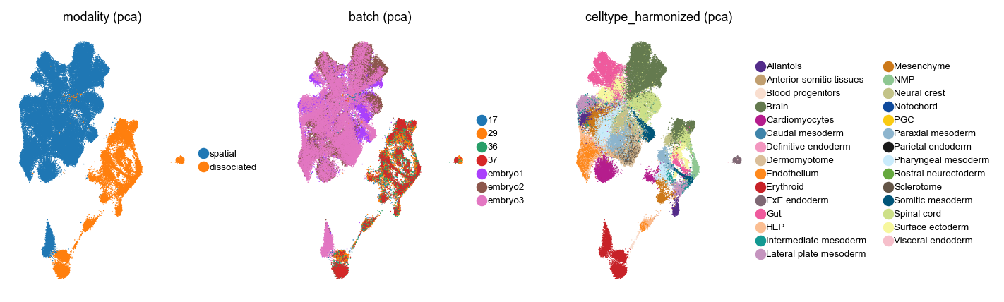
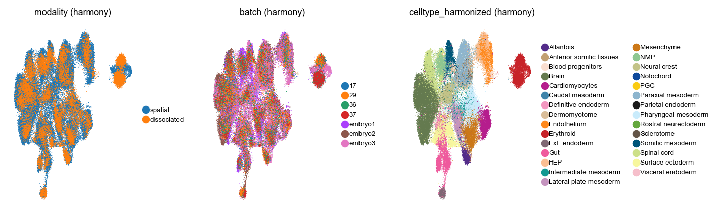
Looks like Harmony aligned both datasets - to make this statement robust and quantitative, we should compute some metrics, like scIB metrics [LButtnerC+22], but for the purpose of this tutorial, let’s just work with this Harmony latent space. We will copy it back into the individual AnnData objects.

ad_diss.obsm["X_harmony"] = ad_combined[ad_combined.obs["modality"] == "dissociated"].obsm["X_harmony"].copy()
ad_sp.obsm["X_harmony"] = ad_combined[ad_combined.obs["modality"] == "spatial"].obsm["X_harmony"].copy()

Work with CellMapper

Initialize and compute the mapping matrix

cmap = cellmapper.CellMapper(query=ad_sp, reference=ad_diss)
cmap

INFO     Initialized CellMapper with 51787 query cells and 16496 reference cells.

CellMapper(query=AnnData(n_obs=51,787, n_vars=351), reference=AnnData(n_obs=16,496, n_vars=18,499)

The central object in CellMapper is the mapping_matrix, which we will use throughout all use cases below.

cmap.compute_neighbors(use_rep="X_harmony", only_yx=True)
cmap.compute_mapping_matrix()

WARNING  Using sklearn for neighbor search with large dataset (16496 cells). Consider using approximate k-NN search
         (e.g. pynndescent) or GPU acceleration (e.g. faiss or rapids)                                             
INFO     Using sklearn to compute 30 neighbors.                                                                    
INFO     Computing mapping matrix using kernel method 'gauss'.

Transfer cell type labels

Let’s pretend we don’t have cell type annotations in the spatial data and we want to transfer them from the dissociated data.

cmap.map_obs(key="celltype_harmonized")

INFO     Mapping categorical data for key 'celltype_harmonized' using direct multiplication.                       
INFO     Categorical data mapped and stored in query.obs['celltype_harmonized_pred'].

Let’s take a look at original and predicted cell type labels for the spatial query data. We’ll take embryo1 as an example.

with warnings.catch_warnings():
    warnings.simplefilter("ignore")

    with plt.rc_context({"figure.figsize": (2, 3), "legend.fontsize": 6, "axes.titlesize": 8}):
        sq.pl.spatial_scatter(
            ad_sp,
            color=["celltype_harmonized", "celltype_harmonized_pred", "celltype_harmonized_conf"],
            library_key="embryo",
            library_id="embryo1",
            shape=None,
            wspace=1.1,
        )

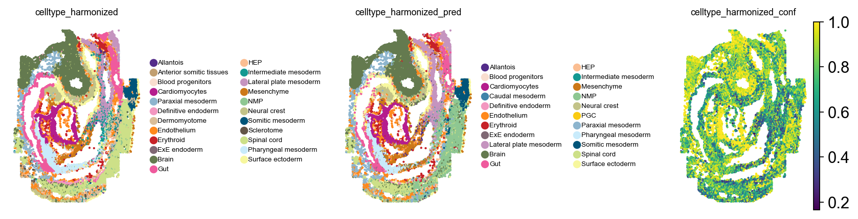
For most cell types, this looks okay. Confidence scores are written to .obs let’s take a look at their distribution:

sns.displot(ad_sp.obs["celltype_harmonized_conf"], kind="kde")

<seaborn.axisgrid.FacetGrid at 0x12a7317f0>

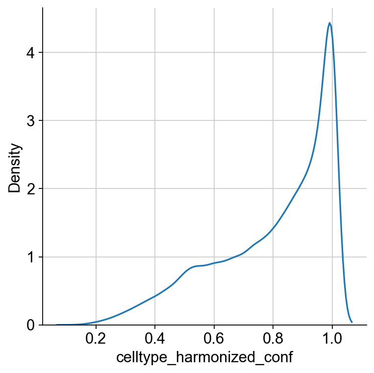
To focus on high-confidence predictions, we could now threshold based on this score. To gain more insights into the mapping on the cell type level, let’s look at a confusion matrix.

cmap.plot_confusion_matrix(pred_key="celltype_harmonized", include_values=False, normalize="true")

<Axes: title={'center': 'Confusion Matrix'}, xlabel='Predicted label', ylabel='True label'>

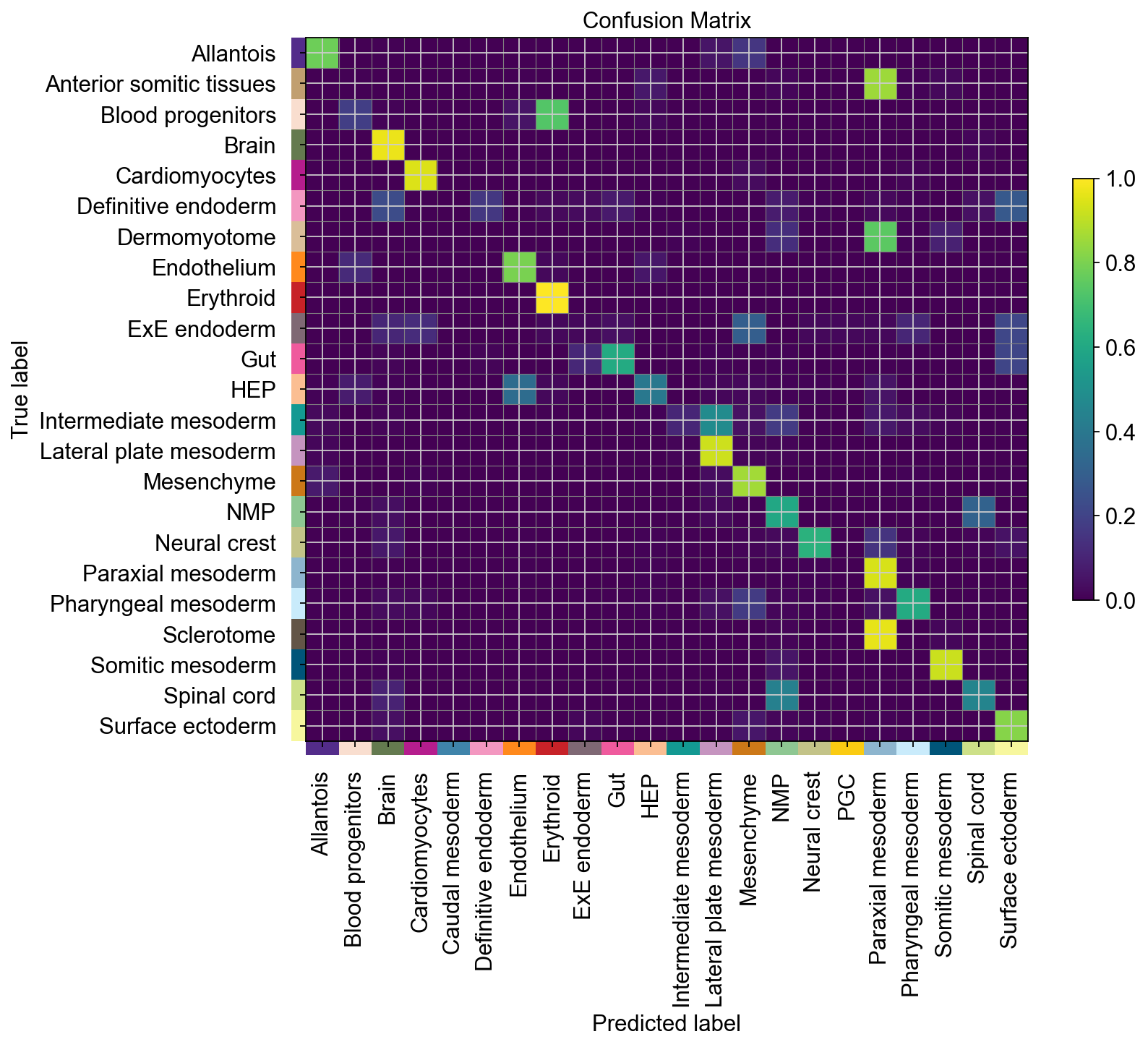
Except for a couple of outliers, some of which map to related tissues, this looks quite good. Let’s quantify this next. For this evaluation, we can threshold based on the confidence score from above.

cmap.evaluate_label_transfer("celltype_harmonized", confidence_cutoff=0.4)

INFO     Accuracy: 0.7283, Precision: 0.7569, Recall: 0.7283, Weighted F1-Score: 0.7180, Macro F1-Score: 0.5242,   
         Excluded Fraction: 0.0414

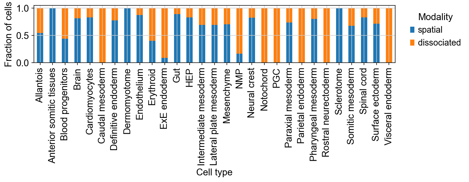
A weighted f1 score of approx. 0.7 on this dataset is pretty good, given that the abundance of certain cell types varies strongly between spatial and dissociated data:

df = ad_combined.obs.groupby(["celltype_harmonized", "modality"], observed=True).size().unstack()
df = df.div(df.sum(axis=1), axis=0)  # each cell type (row) sums to 1
ax = df.plot(kind="bar", stacked=True, figsize=(10, 4))
ax.set_ylabel("Fraction of cells")
ax.set_xlabel("Cell type")
ax.legend(title="Modality", bbox_to_anchor=(1.02, 1), loc="upper left", frameon=False)
plt.tight_layout()
plt.show()

Transfer expression values

We have many more genes measured in the dissociated dataset, so let’s impute their expression in space. We’ll adjust the library size of the imputed data using the empirical library size in space, only considering train genes.

# compute the target library size
target_libsize = ad_sp[:, ad_sp.var.query("is_train").index].layers["counts"].sum(axis=1).A1

# map expression
cmap.map_layers(key="counts", target_libsize=target_libsize)

# evaluate expression transfer on the test genes
cmap.evaluate_expression_transfer(
    layer_key="counts", groupby="embryo", comparison_method="pearson", test_var_key="is_test"
)

INFO     Mapping layer for key 'counts' using direct multiplication                                                
INFO     Imputed expression matrix with shape (51787, 18499) converted to AnnData object.                          
         Observation metadata from query and feature metadata from reference were linked (not copied).             
INFO     Successfully adjusted library sizes for layer 'counts'.                                                   
INFO     Expression for layer 'counts' mapped and stored in query_imputed.X.                                       
         Note: The feature space matches the reference (n_vars=18499), not the query (n_vars=351).                 
INFO     Expression transfer evaluation (pearson): average value = 0.3600 (n_shared_genes=350, n_test_genes=50)    
INFO     Metrics per group defined in `query.obs['embryo']` computed and stored in `query.varm['metric_pearson']`

Depending on the held out genes set, you shoud see an average pearson corrleation of about 0.4 across test genes, which is pretty good for this datset.

To make this comparison robust, we would have to use k-fold cross validation though, to make sure the random gene set does not influence our results. We can look into the mean correlation per embryo on test genes now.

ad_sp[:, ad_sp.var["is_test"]].varm["metric_pearson"].mean()

embryo1    0.333957
embryo2    0.350511
embryo3    0.375450
dtype: float32

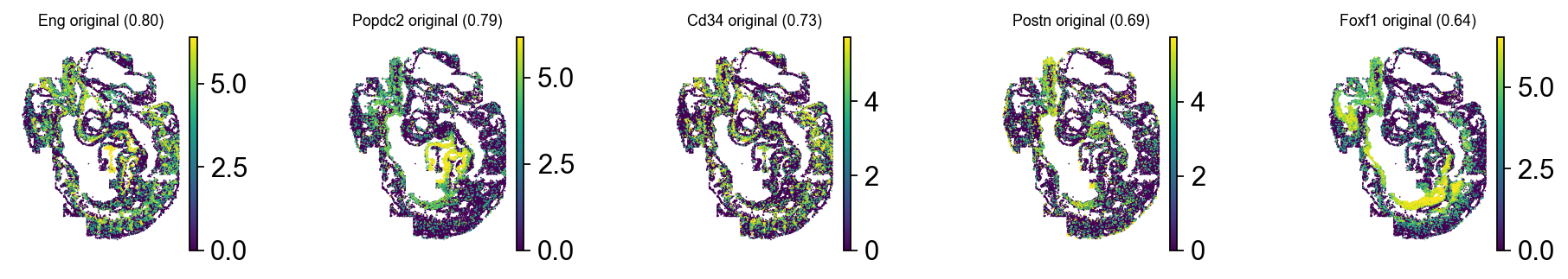
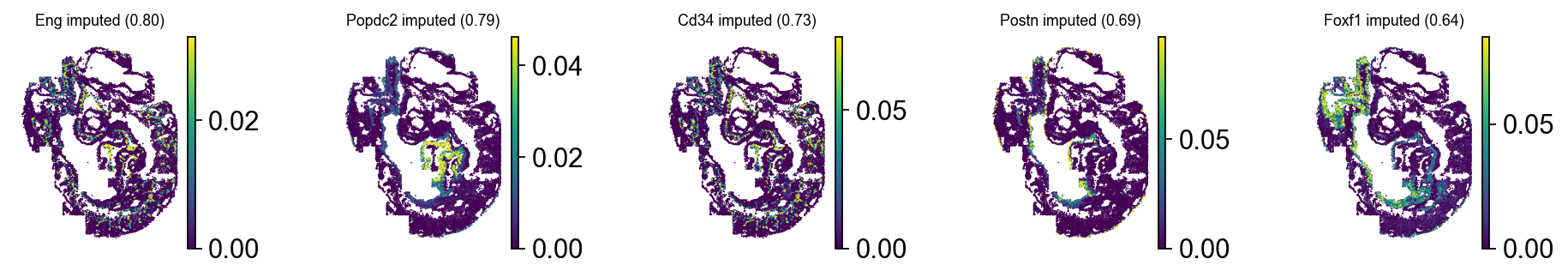
It looks like this worked best on embryo3, so let’s visualize imputed (written to .query_imputed) and original gene expressio of some (held out) test genes for this embryo. We’ll use scanpy here as it allows us to specify a percentile for plotting via vmax.

obs_mask = ad_sp.obs["embryo"] == "embryo3"
gene_series = (
    ad_sp[:, ad_sp.var["is_test"]].varm["metric_pearson"].sort_values("embryo3", ascending=False).head(5)["embryo3"]
)
gene_names = gene_series.index.tolist()
gene_corrs = gene_series.values

with warnings.catch_warnings():
    warnings.simplefilter("ignore")
    with plt.rc_context({"figure.figsize": (2, 2), "legend.fontsize": 6, "axes.titlesize": 8}):
        for adata, key in zip([ad_sp[obs_mask], cmap.query_imputed[obs_mask]], ["original", "imputed"], strict=False):
            sc.pl.spatial(
                adata,
                spot_size=2,
                color=gene_names,
                title=[f"{name} {key} ({corr:.2f})" for name, corr in zip(gene_names, gene_corrs, strict=False)],
                ncols=len(gene_names),
                size=2,
                vmax="p99",
            )

CellMapper supports further metrics to compare transferred expression, such as spearman correlation or Jensen–Shannon divergence.